Gerrit VanderWaal
Sometimes I give myself research projects and this is where I write up my findings.
emailgithub
openstreetmap
Where do apples like to grow?
Finding optimal orchard locations with a geospatial suitability analysis
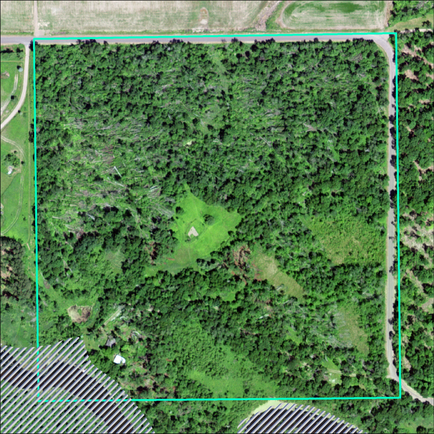
A derecho blasted through my friend's family's cabin property on July 19, 2019. Several months ago, a majority of the property was clear-cut in order to remove the downed trees. Naturally, there's some debate about what to do with the significant increase in unforested land, but one of the planned uses was an orchard. My friend was aware of my mapping/geology background and asked me to plot some figures during the design process.
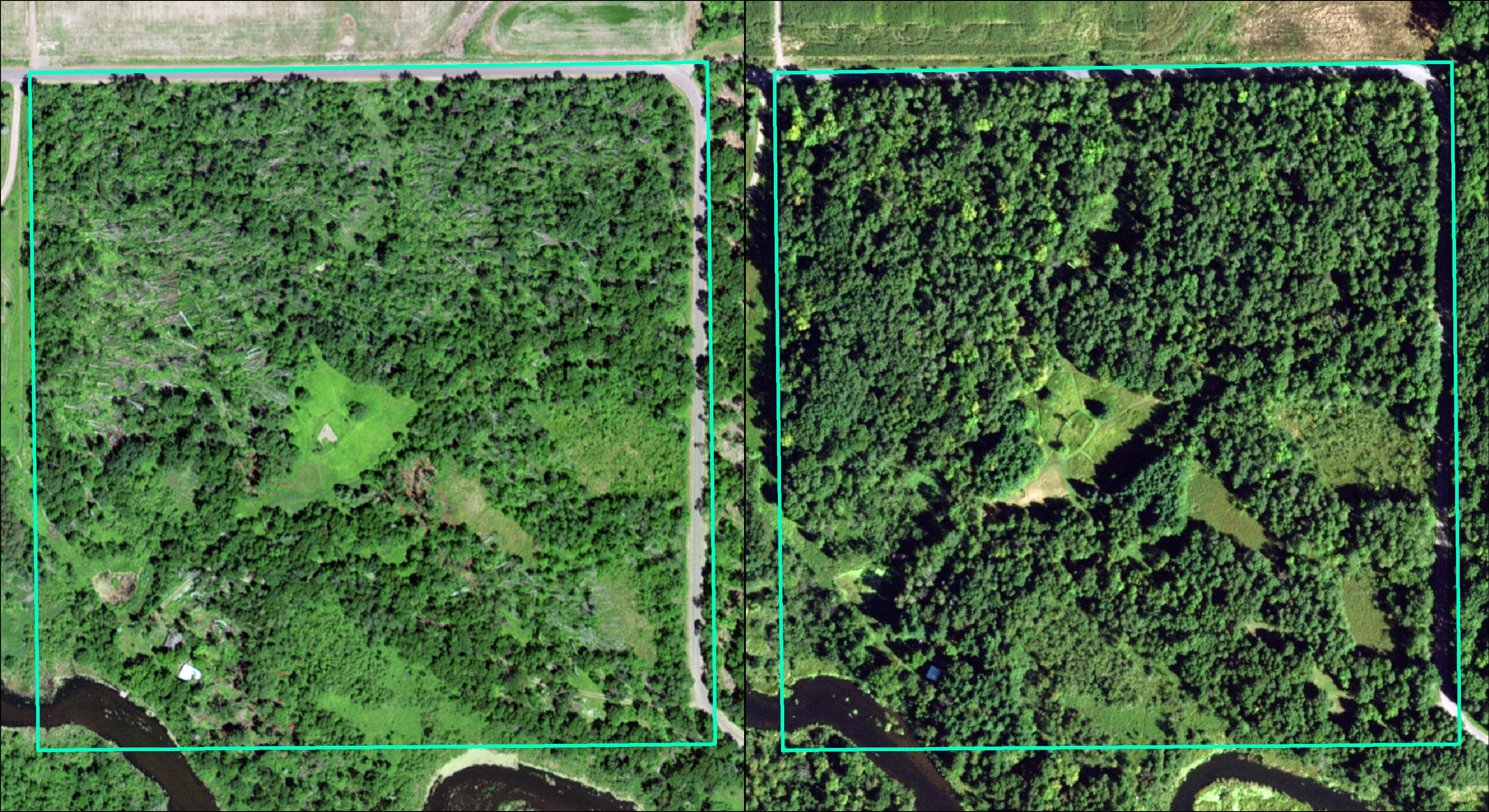
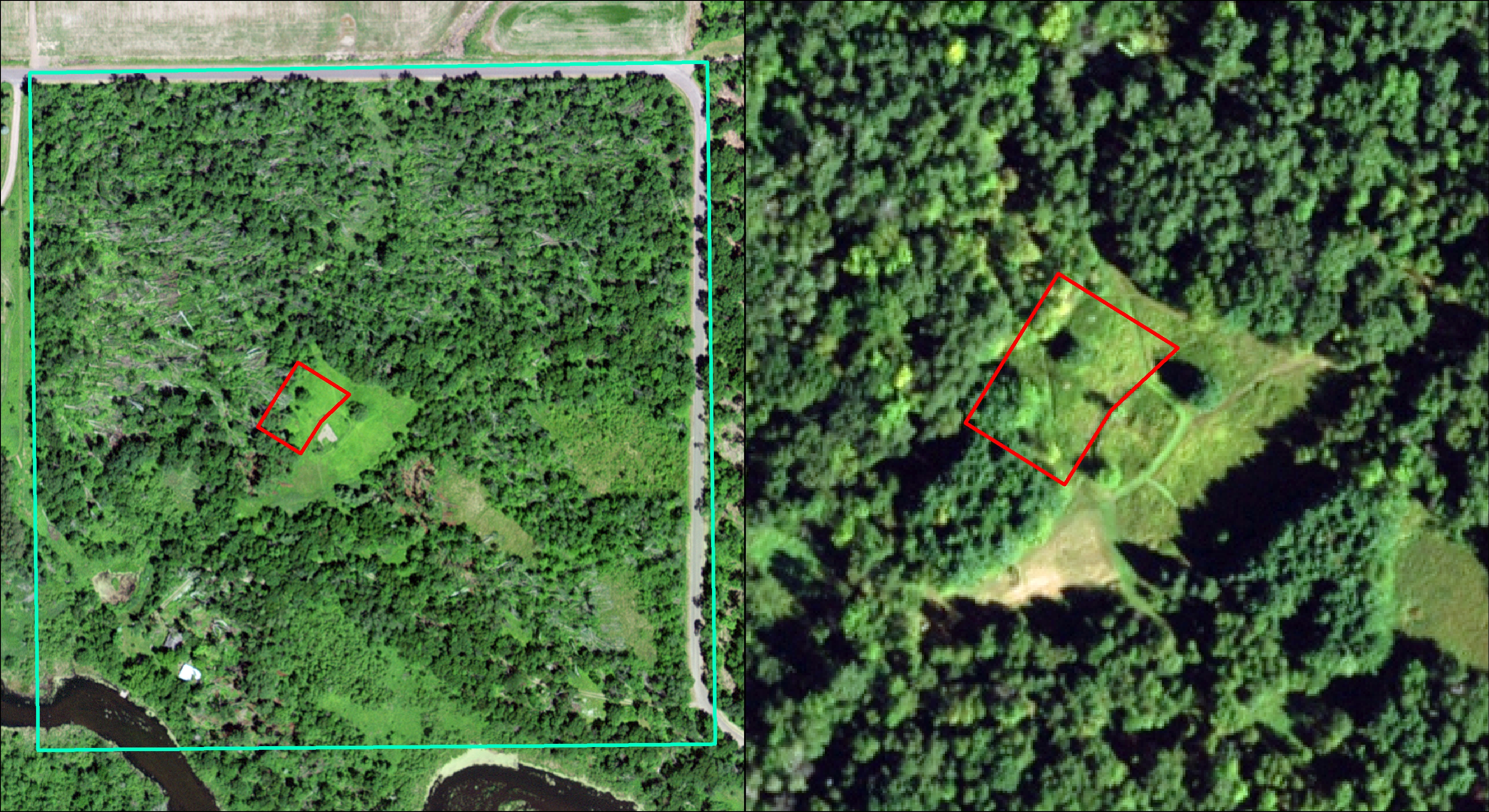
During that process I was inspired to conduct a suitability analysis to see if there were other areas of the property that might be optimally suited for an orchard. As currently designed, the orchard was to be situated adjacent a garden established by one of the former property owners.
A suitability analysis consolidates different datasets with the intent of modeling ideal locations for a use, in this case an orchard. For this analysis we'll rely on the Weighted Overlay tool provided with Esri's ArcMap software. Using Weighted Overlay looks something like this:
- Identify a goal (find alternate locations that are best suited for an orchard)
- Identify attributes that would assist in achieving that goal
- Acquire or create geospatial datasets of those attributes
- Rank the data in terms of desirability using a common scale (e.g. 1-5 with 5 being most optimal)
- Assign weights to the datasets (how important the dataset is to an optimal outcome)
- Run Weighted Overlay
- Analyze result
Research
Since we've established our goal, we'll establish our scope. Because an orchard is defined as any plot of land where fruit or nut trees are grown, we’ll narrow the scope to an apple orchard. We won’t narrow the scope to any particular cultivars. We'll focus on doing relatively surface-level research given financial and time constraints. Next, we'll identify attributes required for a successful apple orchard.
I don’t know anything about growing apples! So I searched the internet. I limited myself to the first several pages of Google for the sake of convenience and speed. I found three primary resources that seem reputable:
- Teryl R. Roper, Daniel L. Maher, and Patricia S. McManus’ Growing Apples in Wisconsin
- Teryl R. Roper & Gary G. Frank’s Planning and Establishing Commercial Apple Orchards in Wisconsin
- Robert Crassweller’s Orchard Establishment - Site Selection and Preparation
For the first two, click “View Publication” instead of paying.
| Growing Apples in Wisconsin | Planning and Establishing Commercial Apple Orchards in Wisconsin | Orchard Establishment - Site Selection and Preparation | |
|---|---|---|---|
| Slope | A “gentle slope” | “Slopes of hills or ridges are generally more desirable than the tops because of wind conditions.” | 4-8% slope |
| Elevation | “...land with a gentle slope so that cold air can settle into adjacent lower areas.” | "...be elevated above surrounding areas...” | “The ideal site is on rolling or elevated land...” |
| pH | 6.0-7.0 | 5.8-6.8 | 6.0-6.5 |
| Drainage | “The soil must have good internal water drainage...” | Orchard soils must be well drained...” | “An old recommendation for a desirable orchard soil is that it be...well drained.” |
| Soil depth | “Most of the active roots are found in the top 12 inches of soil...” | “If water stands within 3-4 feet of the surface...the site is probably unsuitable for an orchard.” | “...minimum of 3 to 4 feet deep.” |
| Organic matter | “Apples grow best in fertile...soils” | "low fertility...soils will almost certainly lead to failure.” | “Soil fertility should be medium to low.” |
| Aeration | “Roots do not tolerate...poorly aerated soils.” | "Orchard soils must be well...aerated.” | — |
| Slope exposure | — | Paragraph 3, page 3 discusses states that due to south-facing slopes receiving more sunlight, temperature fluctuations in winter are greater as a result, leading to tree damage | “Slope exposure should be considered for its effect on fruit trees as they come out of dormancy. A southern-facing slope warms up faster in spring, while the opposite is true of a northern slope. Eastern-facing slopes are intermediate.” |
| Water-holding capacity | Paragraph 8, page 5 implies water-holding capacity is a beneficial soil attribute. | "Soils with good water-holding capacity will retain moisture and supply water to trees during dry periods.” | — |
| USDA Zone | — | "[In USDA Zone 3] apple production is marginal and site selection becomes even more important.” | — |
The soil fertility recommendations do not agree and bear further research, as does soil aeration, aspect (the direction a slope faces), and USDA Zone. I feel confident assuming the importance of water-holding capacity based on the information available.
Soil Health in Orchards claims agricultural soils average 1-6% organic matter but does not cite a source. Table 2 of an academic study records percentages ranges from 1-4ish%, but only from a single orchard. While many resources reiterate the importance of soil organic matter, few (reliable) sources provide quantitative recommendations, so for the sake of convenience we’ll go with 2-6% as the ideal amount of soil organic matter.
T.T. Kozlowski’s Soil Aeration, Flooding, and Tree GrowthPDF, 1.1 MB lists a multitude of reasons why soil aeration is a good thing but does not list quantitative measurements, nor is it strictly about apples, but I think it’s usable enough to inform our analysis.
Site Assessment, Selection and Development for Perennial Crops GuidePDF, 0.15 MB recommends south-facing slopes due to greater exposure to sunlight, as does Growing Fruit Trees in MontanaPDF, 1.5 MB. However, Starting a Community Orchard in North DakotaPDF, 1.9 MB recommends against south-facing slopes due to increased likelihood of breaking winter dormancy due to winter temperature fluctuations, which may also cause sunscalding and trunk cracking. While it would be nice to place the trees so that they receive more sunlight and therefore grow more quickly, tree damage would occur at any stage of the tree's growth, and so we'll consider a north-facing slope ideal.
USDA zone preference likely depends on the cultivar chosen and this can be disregarded.
Data
Aerial imagery
A variety of aerial imagery was used as references, either for figure creation or creation of geospatial data. They include:
- 1938, August 18: United States Department of Agriculture (USDA) via the University of Wisconsin-Madison's WHAIFinder service
- 1979, May 24: USDA via the United States Geological Survey (USGS)'s EarthExplorer service
- 1996, May 18: Polk County via EarthExplorer
- 2010, April 4: North Central Wisconsin Regional Planning Commission via EarthExplorer
- 2018, September 6: USDA National Agriculture Imagery Program (NAIP) via EarthExplorer
- 2020, June 25: USDA NAIP via EarthExplorer
Buildings and roads
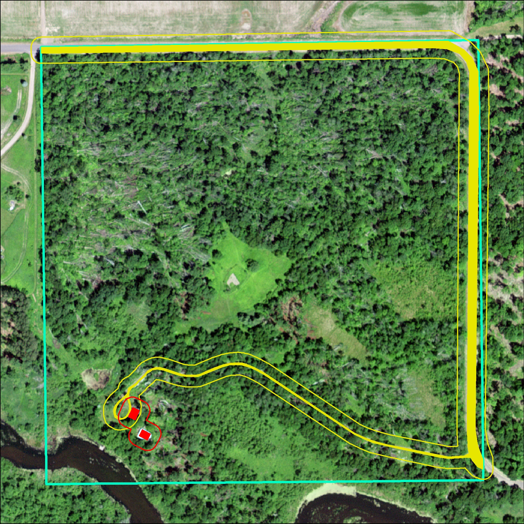
Buildings and roads were heads-up digitized using a combination of the slope raster and the leaf-off 2010 aerial imagery as references. The Polk County GIS Division publishes road centerlines, but these are not helpful for our use-case. To lessen the annoyance from storm damage, we'll restrict trees from being planted from within 30 feet of buildings and roads. 30ft is the approximate maximum apple tree height (based off a quick review of Google sources), but it’s probable the chosen cultivar will be much shorter than this to aid fruit harvesting.
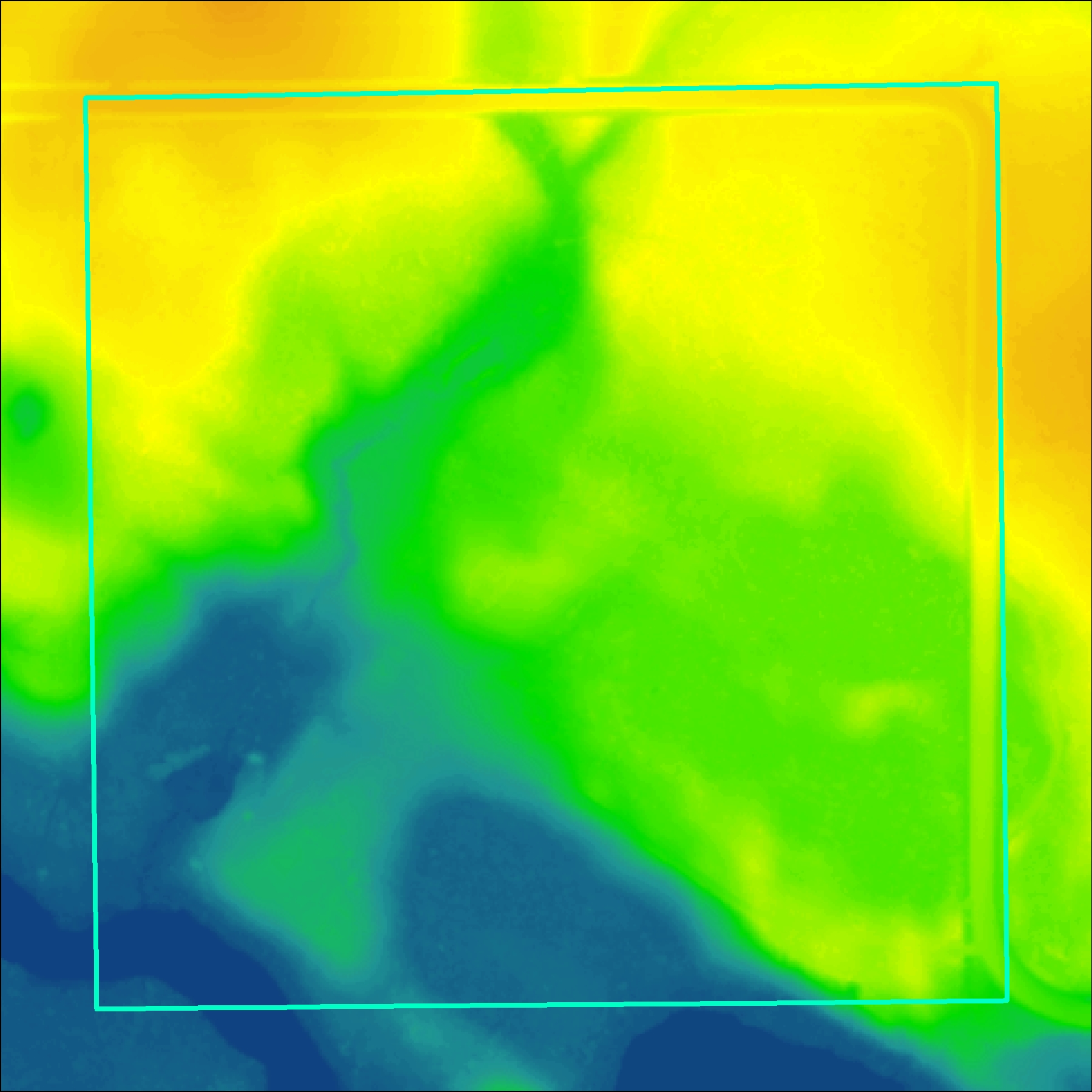
Elevation
Elevation data is commonly delivered in a raster format called a Digital Elevation Model (DEM). I located three DEM sets we could choose from: two acquired for the USGS's 3D Elevation Program (3DEP, 2016) and one LiDAR (Light Detection and Ranging) flown for Polk County (2015). While the 3DEP DEMs are more recent and thus would better match ground conditions, at 1 arc-second (~30 meter) resolution and 1/3 arc-second (~10m) they're far too coarse for our use case. Resolution refers to how much ground a given raster cell represents — in the case of the latter 3DEP set, one cell represents a 10m-by-10m square on the ground. The Polk County 2015 will be used (1m resolution!), and from this we can derive slope and aspect. DEM tiles were downloaded from the Wisconsin State Cartographer's Office interactive LiDAR tile index for Polk County. This set was acquired any time between March 21-31, 2015; unfortunately, the County's chosen contractor did not provide date metadata on a per-tile basis (or it's not public).
The National Oceanic and Atmospheric Administration maintains a very useful catalogue of the United State's elevation data if you're interested in elevation data for your area.
Floodplain
100-year floodplain polygons were downloaded from the Polk County GIS Division. This were visually validated against FEMA’s web map and the official PDF map. The floodplain map is effective September 16, 2011.
Property boundaries
Parcel data were acquired from the Polk County GIS Division and used to identify the boundary of the property. Validation of property boundaries would require a survey and is out of scope for this analysis. These data were downloaded August 29, 2021.
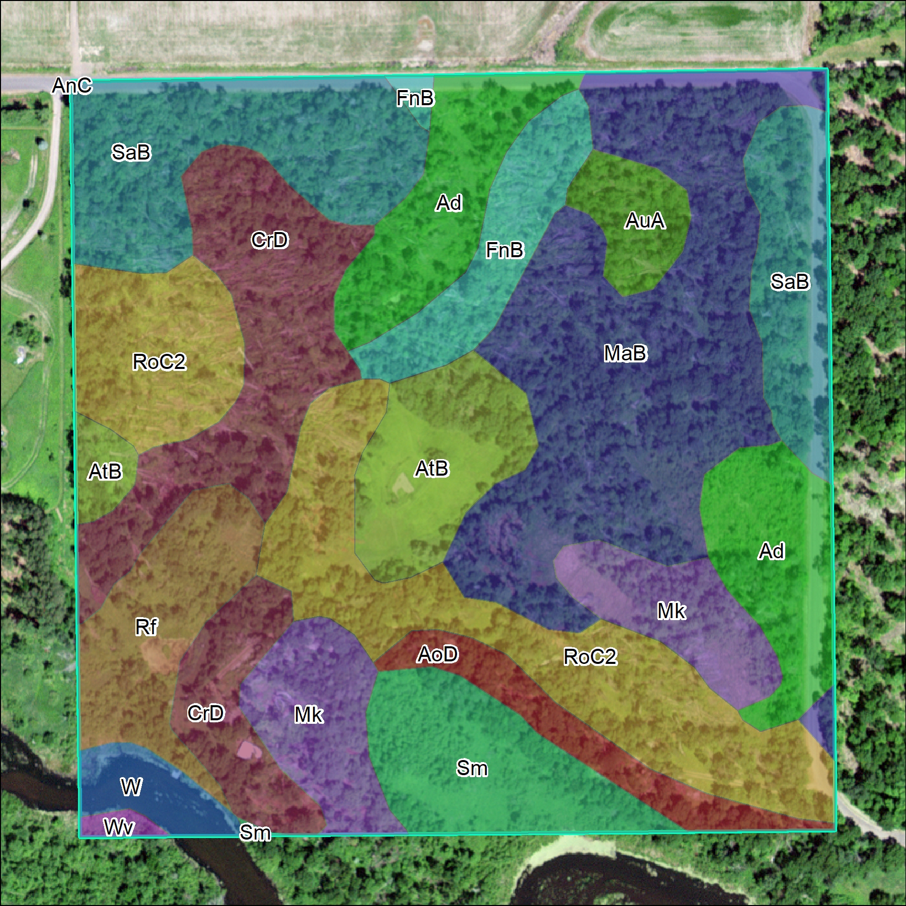
Soil
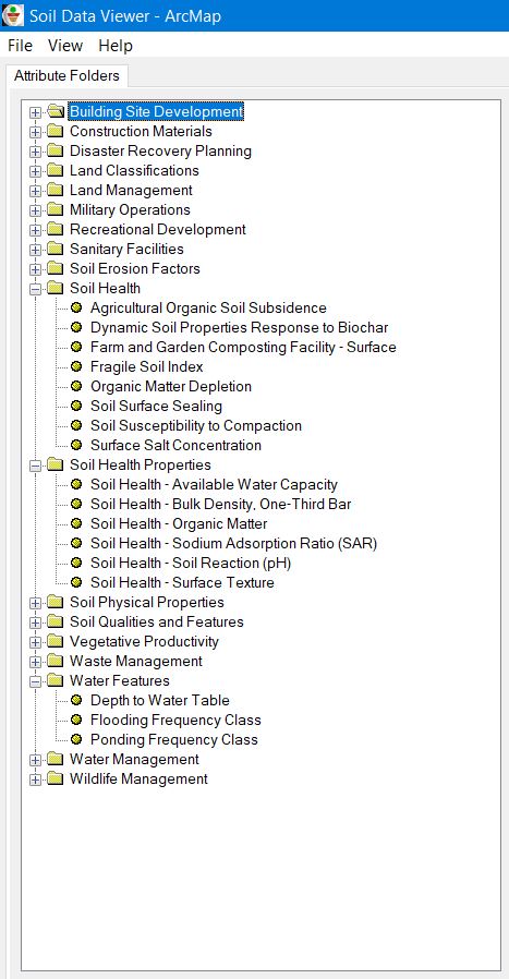
Soil data were downloaded from the Natural Resources Conservation Service (NRCS)’s Web Soil Survey. This generated a product that included polygons of soil unit outlines and tabular data describing various soil attributes. The NRCS’ Soil Data Viewer add-in for ArcMap was used to generate polygons describing each soil unit’s available water capacity (previously referenced as water-holding capacity), depth to water table, drainage class, and organic matter content. A subset of the data available through the add-in can be viewed in this image. I tried to only use “primary” soil attributes, or attributes intrinsic to the soil. For example, the Soil Data Viewer has a “Pesticide Leaching Potential” layer that could be very useful in this analysis, but I figured this Potential would be calculated using primary soil attributes, and therefore would effectively count those soil attributes twice. Additionally, only attributes with values for all soil polygons were used. This data was current as of September 9, 2021.
Wetlands
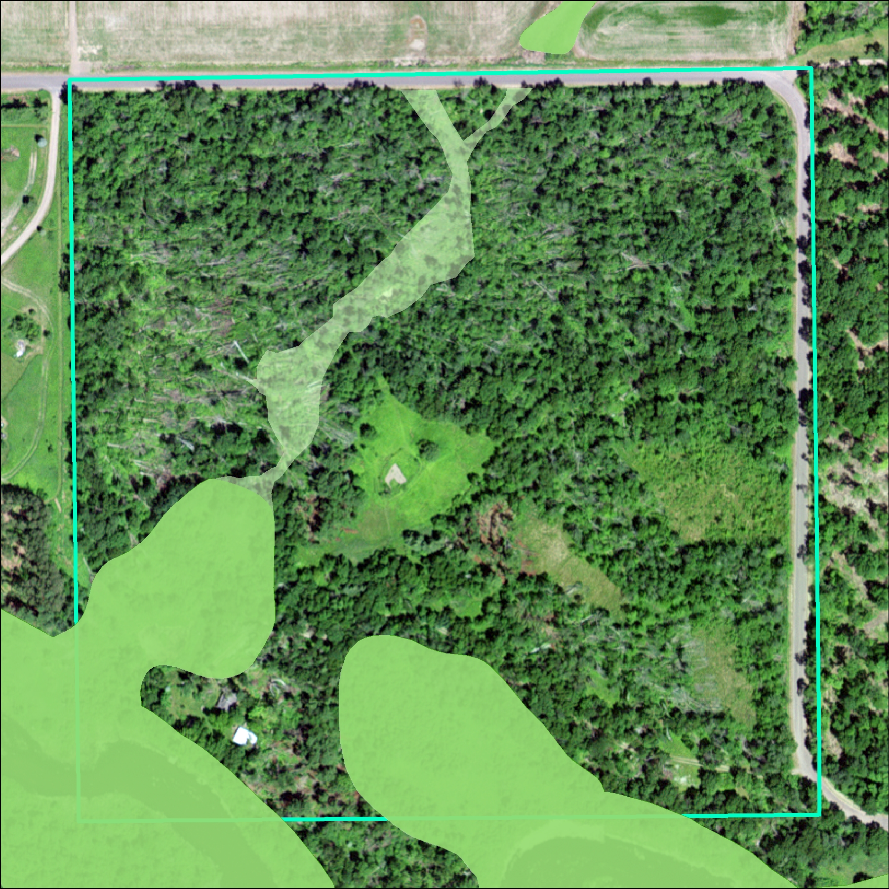
Wetland polygons derived from the Wisconsin Department of Natural Resources Wetland Survey were downloaded from the Polk County GIS Division and visually validated against the DNR’s web map. These data were augmented by heads-up digitization of an ephemeral stream channel and its floodplain. This feature is not at all apparent when viewing aerial imagery or the wetlands data, but I personally observed it when walking the property and my suspicions were confirmed when viewing the slope raster. It is especially evident in the 1947 aerial imagery.
Processing
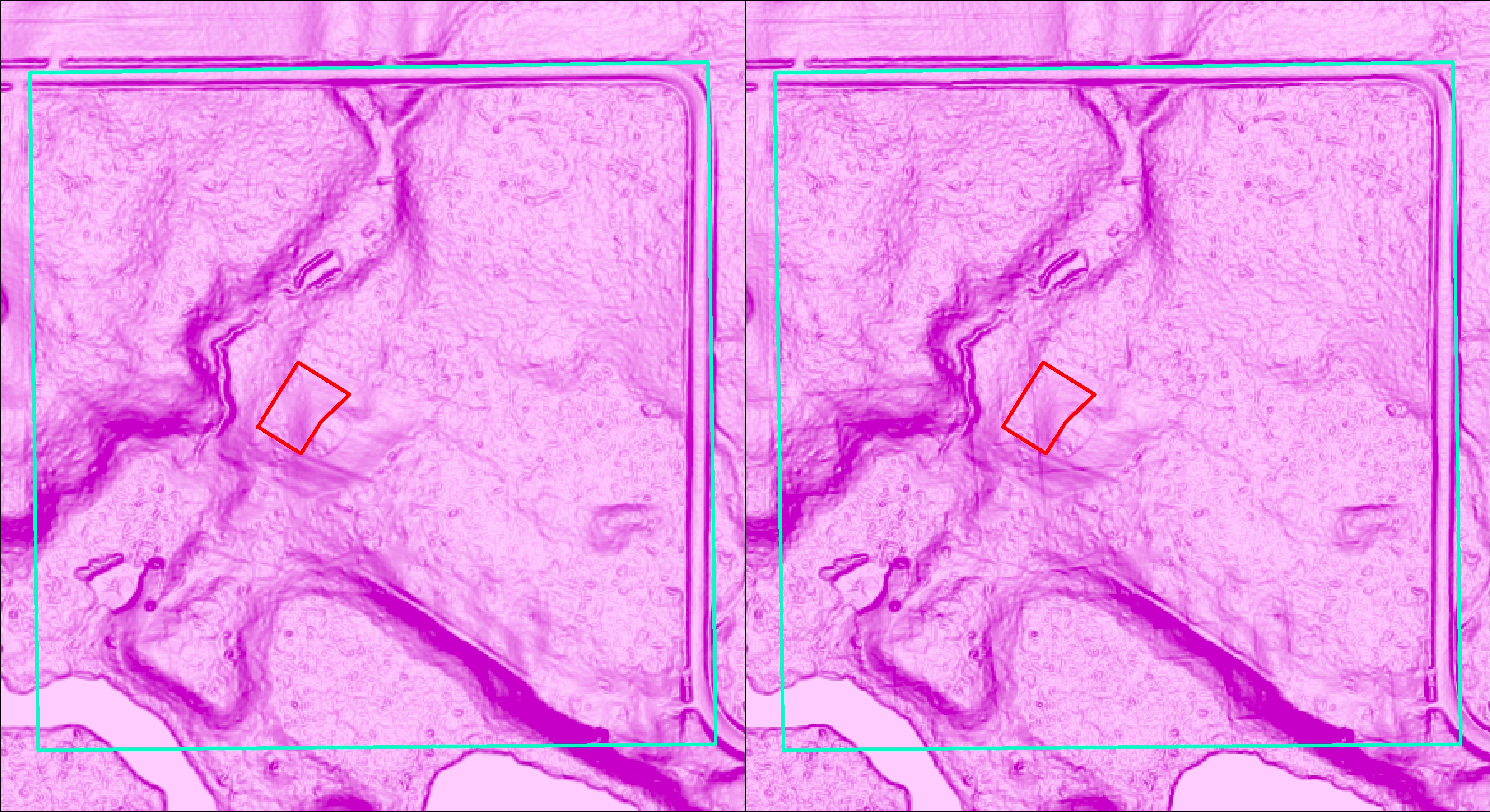
After all primary data (DEMs, soil, etc.) were downloaded they were re-projected in NAD83 UTM Zone 15N. Bilinear resampling was used during the re-projection process to reduce the presence of linear artifacts in the output rasters.
Since the property fell on a seam line between two DEM tiles, they were merged together, then clipped using the property boundary polygon. From this elevation raster, the Slope and Aspect tools were used to generate slope and aspect rasters. The elevation, slope, and aspect tools were then Reclassified to 1) assign weights to the values in the raster and 2) convert the raster to an integer pixel type for use in the Weighted Overlay tool.
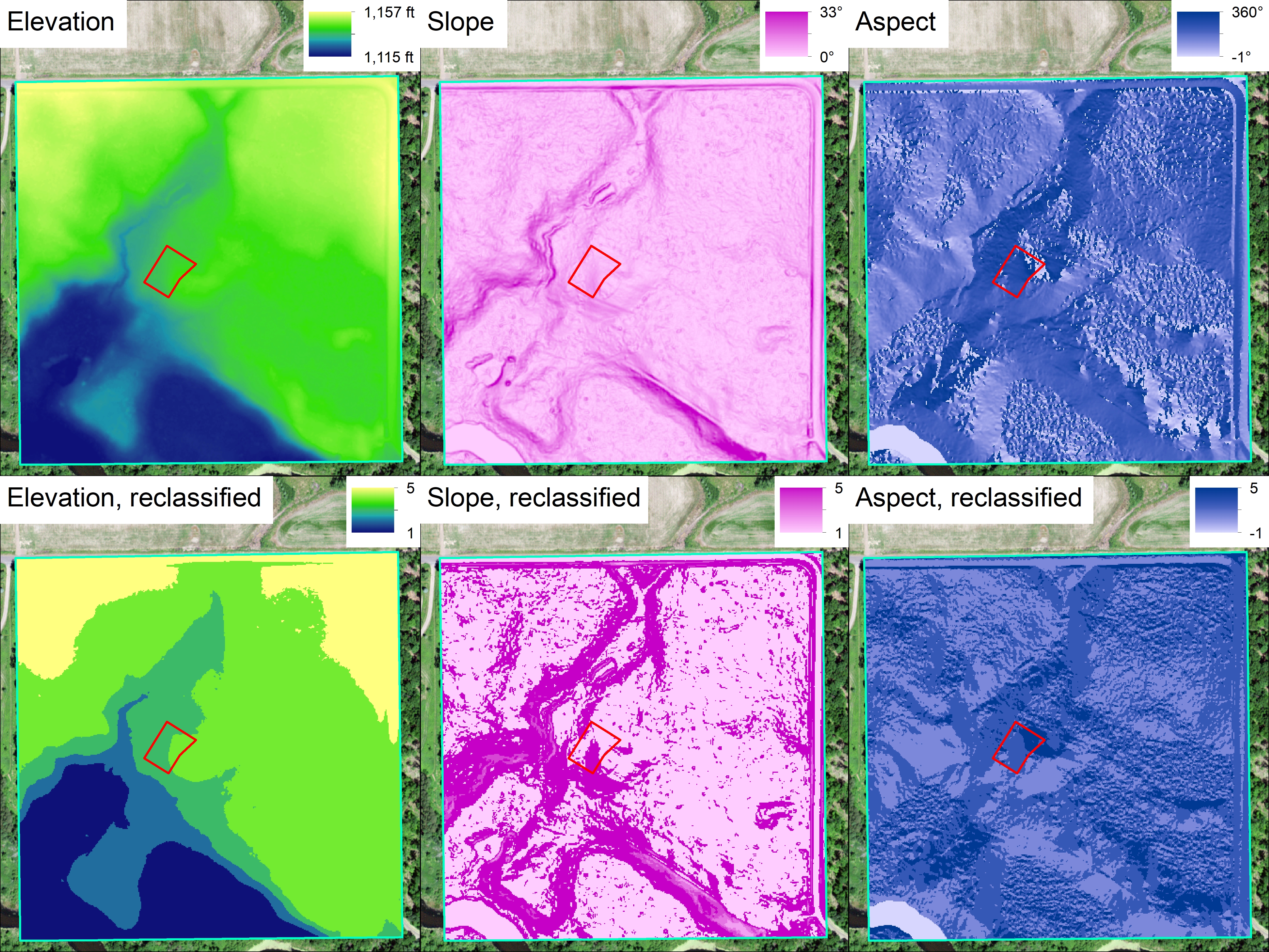
| Elevation (feet) | Slope (°) | Aspect (°) | |||
|---|---|---|---|---|---|
| 1,115-1,123 | 1 | 0-4 | 1 | 135-225 | 1 |
| 1,123-1,132 | 2 | >25 | 2 | — | 2 |
| 1,132-1,140 | 3 | 20-25 | 3 | 45-135; 225-315 | 3 |
| 1,140-1,149 | 4 | 15-20 | 4 | — | 4 |
| 1,149-1,157 | 5 | 4-15 | 5 | 0-45; 315-360 | 5 |
| — | Restricted | — | Restricted | -1 | Restricted |
Weights for elevation are straightforward – the literature suggests planting trees at elevation to avoid areas where cold air will pool. For similar reasons, the literature advises planting trees on a slope, but given the lack of information, I’ve defined “gentle” to incorporate the only quantitative numbers, plus a little more. One could just as easily interpret “gentle” to mean anything up to 45°. Aspect is also self-explanatory: the higher weights are assigned to north-facing slopes to reduce harm during winter. An aspect of -1°, or flat, was only calculated for the river.
Buildings, floodplains, roads, and wetlands were treated identically. The polygons were clipped using the property boundary, converted to rasters with a 1m resolution, and reclassified.
| Buildings | Floodplains | Roads | Wetlands | ||||
|---|---|---|---|---|---|---|---|
| — | 1 | — | 1 | — | 1 | — | 1 |
| — | 2 | — | 2 | — | 2 | — | 2 |
| — | 3 | — | 3 | — | 3 | — | 3 |
| — | 4 | — | 4 | — | 4 | — | 4 |
| NODATA | 5 | NODATA | 5 | NODATA | 5 | NODATA | 5 |
| 1 | Restricted | 1 | Restricted | 1 | Restricted | 1 | Restricted |
Not only are the soils in floodplains and wetlands unsuited for growing apple trees, it would be financially unwise. For floodplains, there’s the obvious chance of the river flooding and your trees being washed away. For wetlands, there are financial penalties for destroying wetlands, or at the very least, legally destroying wetlands would likely be financially prohibitive. Anything not a floodplain or wetland is considered optimal.
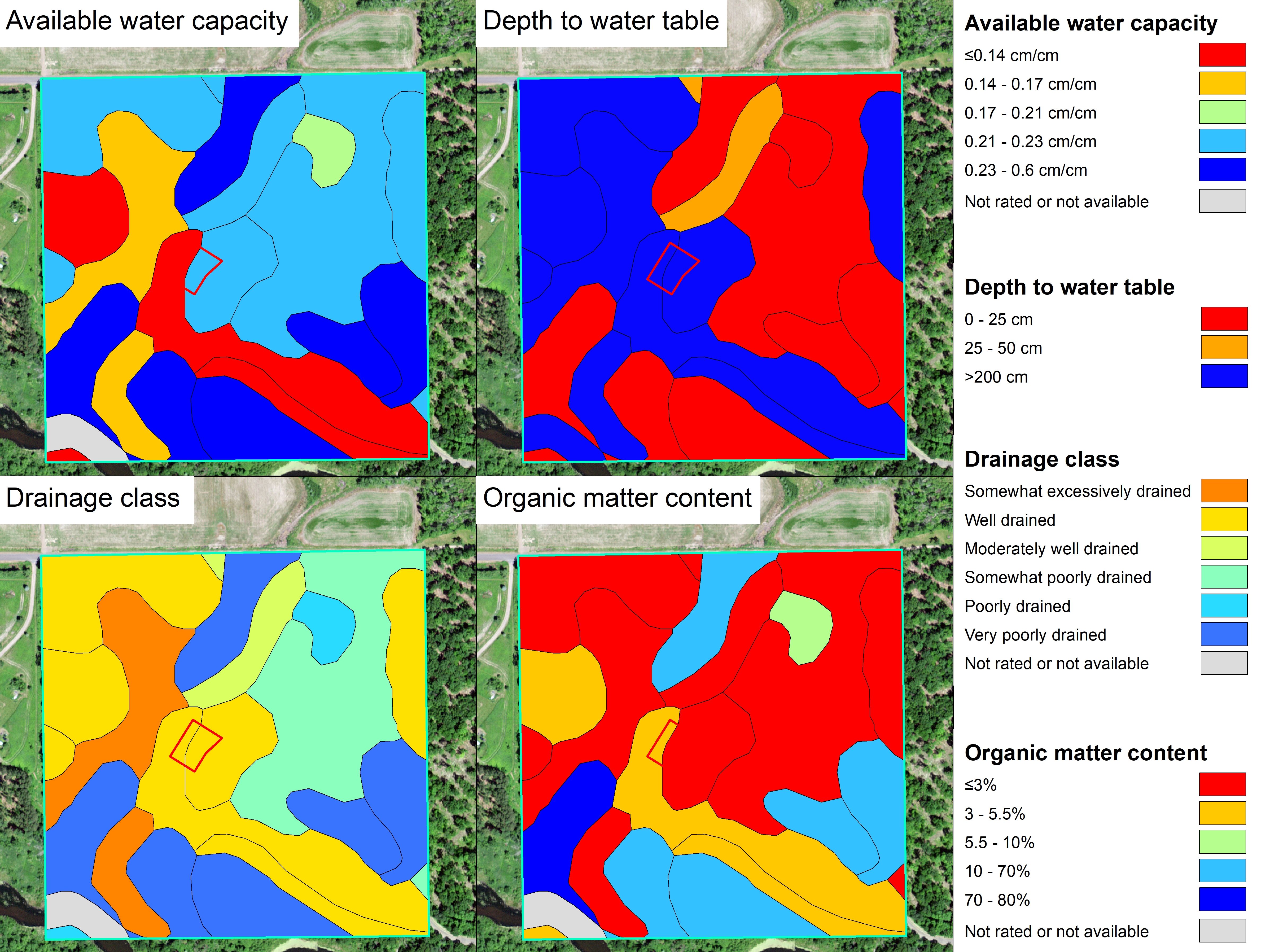
The downloaded soil polygon layer was clipped using the property boundary and the Soil Data Viewer was used to generate available water capacity, drainage class, organic matter content, and depth to water table layers, which were then converted to rasters and reclassified.
| Available water capacity (cm/cm) | Depth to water table (cm) | Drainage class | Organic matter content (% by weight) | ||||
|---|---|---|---|---|---|---|---|
| ≤0.14 | 1 | 0 | 1 | Very poorly drained; Somewhat poorly drained; Poorly drained | 1 | >60 | 1 |
| 0.15-0.17 | 2 | 15 | 2 | — | 2 | — | 2 |
| 0.18-0.21 | 3 | 30 | 3 | Somewhat excessively drained | 3 | 10 | 3 |
| 0.22-0.23 | 4 | — | 4 | Moderately well drained | 4 | 1.25 | 4 |
| 0.23-0.6 | 5 | 201 | 5 | Well drained | 5 | 2-6 | 5 |
| — | Restricted | — | Restricted | — | Restricted | — | Restricted |
In addition to assigning weights to the data, one must assign weights to each layer such that they sum to 100%. We will use these:
| Aspect | 20% |
| Depth to water table | 20% |
| Elevation | 20% |
| Slope | 20% |
| Drainage class | 10% |
| Organic matter content | 5% |
| Available water capacity | 5% |
| Buildings | 0% |
| Floodplain | 0% |
| Roads | 0% |
| Wetland | 0% |
The data that are the least easy to artificially alter have the highest weights, while those that can be artificially altered have lowest. Buildings, floodplains, roads, and wetlands are included exclusively to restrict land from being considered and have the lowest weights of all.
Result
This is the output of running Weighted Overlay!
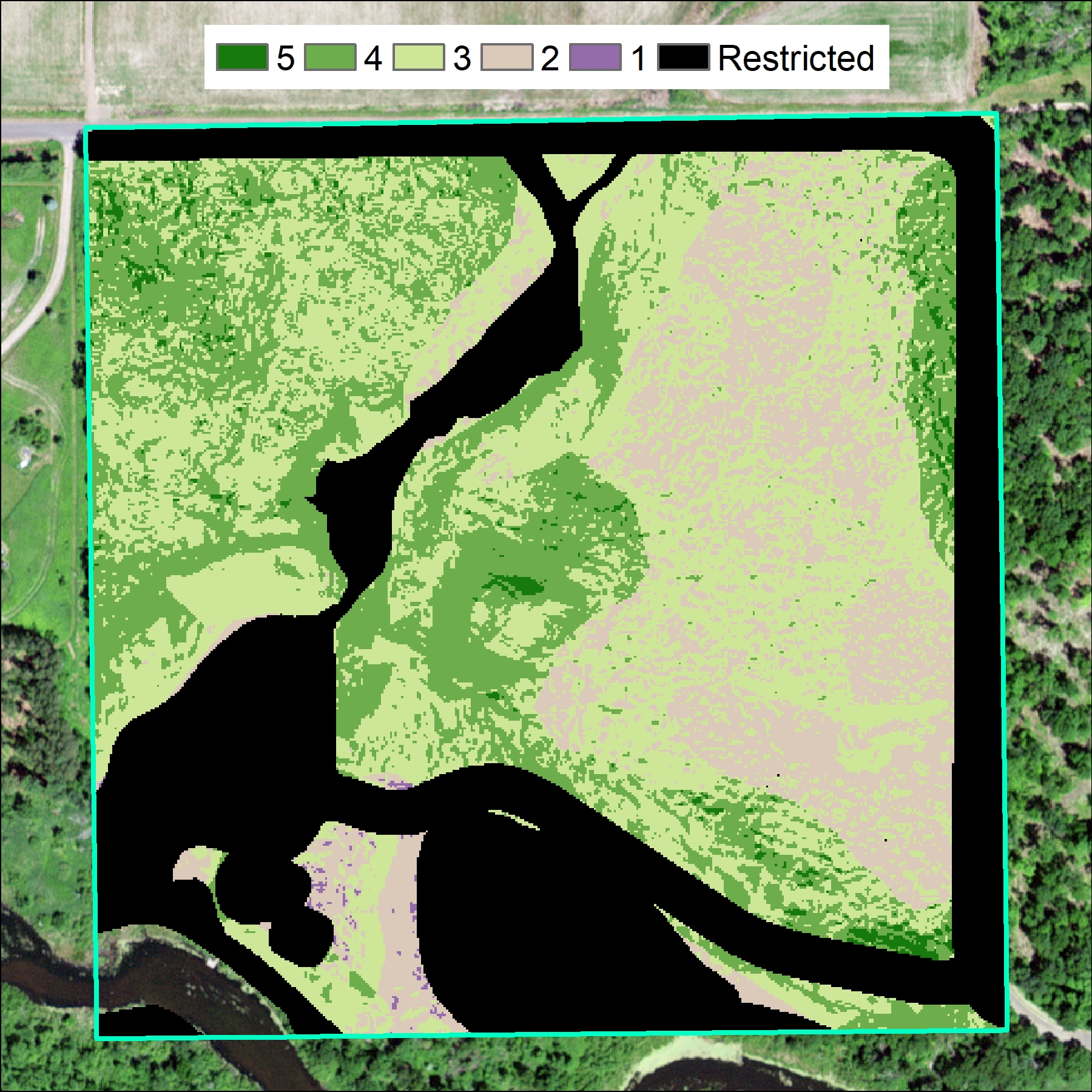
Land calculated as most optimal (5) is finely dispersed but generally restricted to a northwest-southeast trend and a lobe at the northeast corner of the property. Next most-optimal land (4) fills sizeable chunks of the property: primarily the northwest quadrant, the center of the property, and an offshoot along the access road. Middling-ranked land (3) is evenly distributed around the whole property unless currently Restricted. 2-ranked land is almost exclusively present on the eastern half with a small crescent between the buildings and river. Least suitable land is scatterd due east of the buildings.
| Rank | Acreage | % of total acreage |
|---|---|---|
| 1 | 0.6 | 0.13 |
| 2 | 5.6 | 13.7 |
| 3 | 13.8 | 33.6 |
| 4 | 8 | 19.4 |
| 5 | 0.48 | 1.2 |
| Restricted | 12.3 | 30.1 |
Discussion
The results
The result of Weighted Overlay indicates under a quarter of the property would be well suited (4- or 5-ranked) for alternate apple tree locations, with most land in the northwest quadrant and the northeast corner. These are also portions of land that are easy to access as both abut established roads and logging trails. Depending on the level of ambition present, the next step should be direct observation of the soil via hole digging and sampling to verify the result accurately represents ground conditions.
I was a bit shocked to discover the general location of the orchard as planned is well-suited for growing apples. The previous homeowner likely sited the former garden with a different crop in mind and leaned on their personal experience. I expected the data would contradict their judgement — perhaps the soil data would reveal the soil was poorly suited for agriculture, for example.
The data
A model is only as good as its data, and the data used in this analysis are high quality based on the resources available to me. These data are commonly used for planning by government agencies and private landowners alike due to ease of access and few restrictions on their use. The bedrock of this model are the elevation and soils data.
The elevation data portrays the property as it existed on the date acquired — that is, as it was six years ago. This is acceptably current. The largest change to the property since acquisition was the clear-cutting, but the DEMs depict the ground elevation, not the tree canopy. The resolution is good enough to identify buildings and roads, and very importantly, the stream channel bisecting the property.
The soils data seem to be reliable. 12 of 23 soil units are classified as Order 2. According to Chapter 4 of the NRCS' Soil Survey Manual, "Orders" are "determined by the field procedures used to identify soil components and place map unit boundaries, the minimum permissible size of map unit delineation, and the kind of map unit to which soil components are aggregated." The Manual indicates Order 2 data is suitable for general agriculture planning (page 273), which this analysis is. From a brief review of the Manual and Google, I was unable to find a reason why a soil unit would be missing an Order, but I assume it's because the field procedures used in generating the data are unknown.
The Manual describes Order 2 as:
Field procedures allow plotting of soil boundaries by observation and by interpretation of remotely sensed data [e.g. aerial imagery, LiDAR; page 238]. The soils in each delineation are identified primarily by traversing [visiting observation points set any distance apart, where the distance is adjusted based on soil boundaries and the variability of its properties; page 264] and transecting [visiting observation points set at fixed distances apart; page 264]. Observations and remotely sensed data are secondary types of documentation. Boundaries are verified at closely spaced intervals. Map units are mostly consociations and complexes but may also include undifferentiated groups or associations. Map unit components are phases of soil series or phases of miscellaneous areas. Map units may also be named for a taxonomic category above the series. Delineations are variable in size, with a minimum of 0.6 hectare to 4 hectares (1.5 to 10 acres), depending on landscape complexity and survey objectives. Contrasting minor components vary in size and amount within the limits permitted by the kind of map unit used. Base map scale is generally 1:12,000 to 1:31,680, depending on the complexity of the soil pattern within the area.
A shortcoming with the floodplain data I would like to see resolved is the lack of 500-year floodplain boundaries. A 100-year floodplain is defined as an area with a 1% annual chance of flooding, so its existence implies the presence of a 500-year floodplain as well — an area with a 0.2% annual chance of flooding. Since high precipitation events are becoming increasingly common due to anthropogenic climate change, knowing the 500-year boundaries is absolutely critical to long-term planning. Just because they're not currently delineated by FEMA doesn't mean it doesn't exist.
Next Steps
- Groundtruthing: Essential if an alternate orchard location is desired, suggested if proceeding with the current location. While the model provides quantitative insight into ideal locations, the actual viability will depend on ground conditions. Additionaly, it would be helpful (but perhaps not financially prudent) to send soil samples to be analyzed for a refined look at soil attributes.
- 500-year floodplain: If the boundaries can be generated relatively easily, it would be preferred to include them in an updated analysis.
- Additional data review: A more thorough look at the data available through Soil Data Viewer would be useful in figuring out why some data is incomplete, like pH or Total Subsidence. Completed data could be used in enhancing the model.